import numpy as np import matplotlib.pyplot as plt import tensorflow as tf import xlrd
DATA_FILE = 'data/fire_theft.xls'
# Step 1: read in data from the .xls file # book = xlrd.open_workbook(DATA_FILE, encoding_override="utf-8") # sheet = book.sheet_by_index(0) # data = np.asarray([sheet.row_values(i) for i in range(1, sheet.nrows)]) # n_samples = sheet.nrows - 1 import pandas as pd # 使用pandas更简便 df = pd.read_excel(DATA_FILE) data = df.values n_samples = len(df.index)
# Step 2: create placeholders for input X (number of fire) and label Y (number of theft) X = tf.placeholder(tf.float32, name='X') Y = tf.placeholder(tf.float32, name='Y')
# Step 3: create weight and bias, initialized to 0 w = tf.Variable(0.0, name='weights') b = tf.Variable(0.0, name='bias')
# Step 4: build model to predict Y Y_predicted = X * w + b
# Step 5: use the square error as the loss function loss = tf.square(Y - Y_predicted, name='loss')
# Step 6: using gradient descent with learning rate of 0.01 to minimize loss optimizer = tf.train.GradientDescentOptimizer(learning_rate=0.001).minimize(loss)
with tf.Session() as sess: # Step 7: initialize the necessary variables, in this case, w and b sess.run(tf.global_variables_initializer()) writer = tf.summary.FileWriter('./my_graph/03/linear_reg', sess.graph) # Step 8: train the model for i in range(100): # train the model 100 times total_loss = 0 for x, y in data: # Session runs train_op and fetch values of loss _, l = sess.run([optimizer, loss], feed_dict={X: x, Y:y}) total_loss += l print'Epoch {0}: {1}'.format(i, total_loss/n_samples)
# close the writer when you're done using it writer.close() # Step 9: output the values of w and b w_value, b_value = sess.run([w, b])
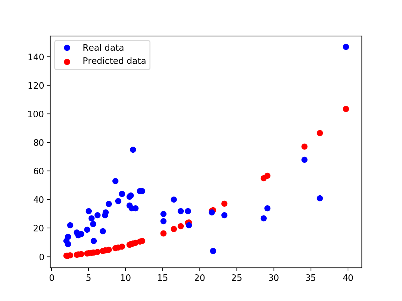
# plot the results X, Y = data.T[0], data.T[1] plt.plot(X, Y, 'bo', label='Real data') plt.plot(X, X * w_value + b_value, 'r', label='Predicted data') plt.legend() plt.show()
100次迭代之后,平均方差还是挺大的,拟合的不够好,所以考虑二次函数 Y = wXX + uX + b。
所以修改第3步和第4步。
1
2
3
4
5
6
7
# Step 3: create weight and bias, initialized to 0
w = tf.Variable(0.0, name='weights_1')
u = tf.Variable(0.0, name="weights_2")
b = tf.Variable(0.0, name='bias')

# Step 4: build model to predict Y
Y_predicted = X * X * w + X * u + b
# coding=utf-8 import numpy as np import matplotlib.pyplot as plt import tensorflow as tf import xlrd
DATA_FILE = 'data/fire_theft.xls'
# Step 1: read in data from the .xls file # book = xlrd.open_workbook(DATA_FILE, encoding_override="utf-8") # sheet = book.sheet_by_index(0) # data = np.asarray([sheet.row_values(i) for i in range(1, sheet.nrows)]) # n_samples = sheet.nrows - 1 import pandas as pd # 使用pandas更简便 df = pd.read_excel(DATA_FILE) data = df.values n_samples = len(df.index)
# Step 2: create placeholders for input X (number of fire) and label Y (number of theft) X = tf.placeholder(tf.float32, name='X') Y = tf.placeholder(tf.float32, name='Y')
# Step 3: create weight and bias, initialized to 0 w = tf.Variable(0.0, name='weights_1') u = tf.Variable(0.0, name="weights_2") b = tf.Variable(0.0, name='bias')
# Step 4: build model to predict Y Y_predicted = X * X * w + X * u + b
# Step 5: use the square error as the loss function loss = tf.square(Y - Y_predicted, name='loss')
# Step 6: using gradient descent with learning rate of 0.01 to minimize loss optimizer = tf.train.AdamOptimizer(learning_rate=0.01).minimize(loss)
with tf.Session() as sess: # Step 7: initialize the necessary variables, in this case, w and b sess.run(tf.global_variables_initializer()) # writer = tf.summary.FileWriter('./my_graph/03/linear_reg', sess.graph)
# Step 8: train the model for i in range(10): # train the model 100 times total_loss = 0 for x, y in data: # Session runs train_op and fetch values of loss _, l = sess.run([optimizer, loss], feed_dict={X: x, Y:y}) total_loss += l
# close the writer when you're done using it # writer.close()
# Step 9: output the values of w and b w_value, u_value, b_value = sess.run([w, u, b])
# plot the results X, Y = data.T[0], data.T[1] plt.plot(X, Y, 'bo', label='Real data') plt.scatter(X, X * X * w_value + X * u_value + b_value, color='r',label='Predicted data') plt.legend() plt.show()
分析代码
通过上面的程序会发现,在创建完优化器后,用 ‘sess.run(optimizer, feed_dict={X: x, Y: y})’ 来运行程序。实际上 TensorFlow 将所有操作作为图的一部分来运算,同时 feed_dict 作为输入的数据,而 loss 是根据 w 和 b 计算得到的,其实 TensorFlow 会根据 loss 来自动求梯度。
import time import numpy as np import tensorflow as tf from tensorflow.examples.tutorials.mnist import input_data
# Step 1: Read in data # using TF Learn's built in function to load MNIST data to the folder data/mnist MNIST = input_data.read_data_sets("/data/mnist", one_hot=True) # Step 2: Define parameters for the model learning_rate = 0.01 batch_size = 128 n_epochs = 25
# Step 3: create placeholders for features and labels # each image in the MNIST data is of shape 28*28 = 784 # therefore, each image is represented with a 1x784 tensor # there are 10 classes for each image, corresponding to digits 0 - 9. # each label is one hot vector. X = tf.placeholder(tf.float32, [batch_size, 784]) Y = tf.placeholder(tf.float32, [batch_size, 10])
# Step 4: create weights and bias # w is initialized to random variables with mean of 0, stddev of 0.01 # b is initialized to 0 # shape of w depends on the dimension of X and Y so that Y = tf.matmul(X, w) # shape of b depends on Y w = tf.Variable(tf.random_normal(shape=[784, 10], stddev=0.01), name="weights") b = tf.Variable(tf.zeros([1, 10]), name="bias")
# Step 5: predict Y from X and w, b # the model that returns probability distribution of possible label of the image # through the softmax layer # a batch_size x 10 tensor that represents the possibility of the digits logits = tf.matmul(X, w) + b
# Step 6: define loss function # use softmax cross entropy with logits as the loss function # compute mean cross entropy, softmax is applied internally entropy = tf.nn.softmax_cross_entropy_with_logits(logits, Y) loss = tf.reduce_mean(entropy) # computes the mean over examples in the batch
# Step 7: define training op # using gradient descent with learning rate of 0.01 to minimize cost optimizer = tf.train.GradientDescentOptimizer(learning_rate=learning_rate).minimize(loss) init = tf.global_variables_initializer() with tf.Session() as sess: sess.run(init) n_batches = int(MNIST.train.num_examples / batch_size) for i in range(n_epochs): # train the model n_epochs times for _ in range(n_batches): X_batch, Y_batch = MNIST.train.next_batch(batch_size) sess.run([optimizer, loss], feed_dict={X: X_batch, Y: Y_batch}) # average loss should be around 0.35 after 25 epochs
# test the model n_batches = int(MNIST.test.num_examples / batch_size) total_correct_preds = 0 for i in range(n_batches): X_batch, Y_batch = MNIST.test.next_batch(batch_size) _, loss_batch, logits_batch = sess.run([optimizer, loss, logits], feed_dict={X: X_batch, Y: Y_batch}) preds = tf.nn.softmax(logits_batch) correct_preds = tf.equal(tf.argmax(preds, 1), tf.argmax(Y_batch, 1)) accuracy = tf.reduce_sum(tf.cast(correct_preds, tf.float32)) # similar to numpy.count_nonzero(boolarray) :( total_correct_preds += sess.run(accuracy) print"Accuracy {0}".format(total_correct_preds / MNIST.test.num_examples)