Machine Learning Note 1

Xin Qiu Jun 02, 2016

Coursera 上的Machine Learning 算得上是经典的机器学习入门课程，是由Andrew Ng大牛上的课。出于对机器学习的好奇，打算用Python来完成这门课的学习。

Supervised learning 监督学习

这里存在两种问题 regression 和 classification。前者是预测相关的问题，后者是分类相关的问题。

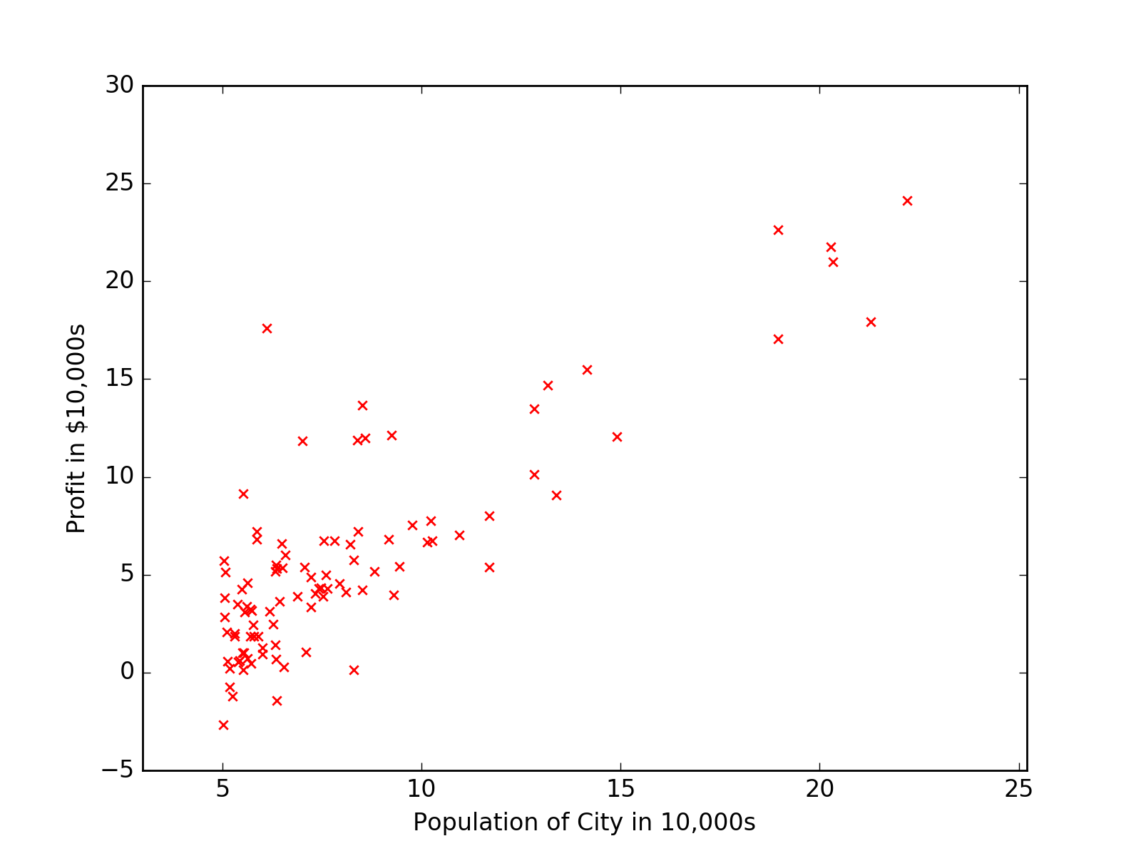
首先介绍的是监督学习，notes1中用房屋价格预测来介绍Linear Regression线性回归。这里因为没有数据集，所以我选择用ex
1中的ex1data1.txt来做演示。

import matplotlib.pyplot as plt
import numpy as np
data = np.loadtxt('ex1data1.txt', delimiter=',')
m = data.shape[0]
X = data[:,0]
y = data[:, 1]
plt.scatter(X, y, c='r', marker='x', linewidths=1)
plt.xlim([3, max(X)+3])
plt.ylabel('Profit in $10,000s')
plt.xlabel('Population of City in 10,000s')
plt.show()

可以画出数据分布散点图。

机器学习的流程如下

          +------------------+
          |                  |
          |     Training     |
          |       set        |
          |                  |
          +------------------+
                   ||
                   ||
          +--------\/--------+
          |                  |
          |     Learning     |
          |     algorithm    |
          |                  |
          +------------------+
                   ||
                   ||
          +--------\/--------+
          |                  |
          |    hypothesis    |
X +------->                  +------->  Y
          |                  |
          +------------------+

用大量的训练数据带入学习算法中进行学习，学习算法产生假设模型，通过假设模型，可以由未知数据X得出需要的Y。

Linear Regression 线性回归

根据 ex1data2.txt 里的数据，因为有两个特征，所以可以写出假设模型

$$ h_{\theta } = \theta_{0}+ \theta_{1}x_{1}+\theta_{2}x_{2}$$

其中 $\theta_{i}$ 是线性方程的确定性参数(有点类似权重的东西？)。所以，假设 $ x_{0} = 1$, 从广义上可以定义假设方程

$$h_{\theta } =\sum_{n}^{i=0}\theta_{i}x_{i}=\theta^{T}x$$

其中 $\theta$ 和 $x$ 都是向量，$n$ 是输入变量的个数。

确定完假设模型，之后需要做的一件事是挑选学习 $\theta$。一个可靠的方法可以让 $h(x)$ 接近 $y$。为了评估假设模型与数据集的接近程度，定义了一个 cost function（代价函数）

$$ J(\theta )=\frac{1}{2}\sum_{m}^{i=1}(h_{\theta}(x^{(i)})-y^{(i)})^{2} $$

这是least-squares cost function，是 ordinary least squares regression model 的一部分。

LMS algorithm

为了寻找合适的 $\theta$ 使 $J(\theta )$ 最小，可以使用LMS算法通过不断的改变 $\theta$ 来寻找合适的值。这里使用了 gradient descent algorithm(梯度递减算法)，更新 $\theta$ 的方式如下

$$ \theta_{j} := \theta_{j} -\alpha \frac{\partial }{\partial \theta_{j}}J(\theta) $$

其中，$\alpha$ 是 learning rate（学习率）, $\frac{\partial }{\partial \theta_{j}}J(\theta)$ 可以化简为
$$ \frac{\partial }{\partial \theta_{j}}J(\theta) = (h_{\theta}(x)-y)x_{j} $$

这样的更新规则称为LMS update rule(least mean squares),也称为Widrow-Hoﬀ learning rule.

$$ \theta_{j} := \theta_{j} + \alpha (y^{(i)} -h_{\theta}(x^{(i)}))x_{j}^{(i)}$$

梯度递减这里提到了两种 batch gradient descent (批量梯度递减) 和 stochastic gradient descent (随机梯度递减)。

Supervised learning 监督学习

Linear Regression 线性回归

LMS algorithm

The normal equations

Reference